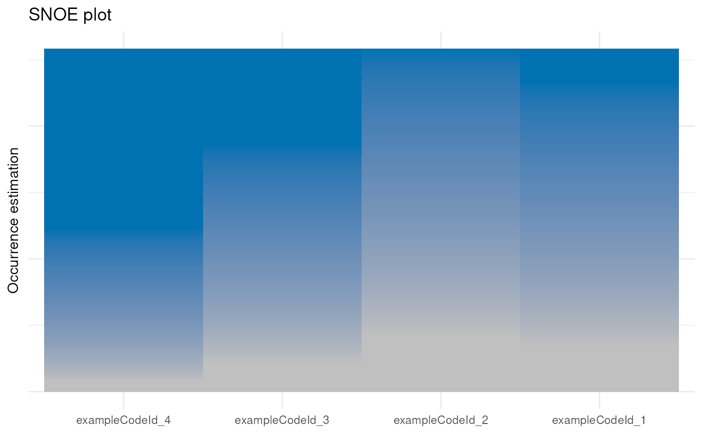
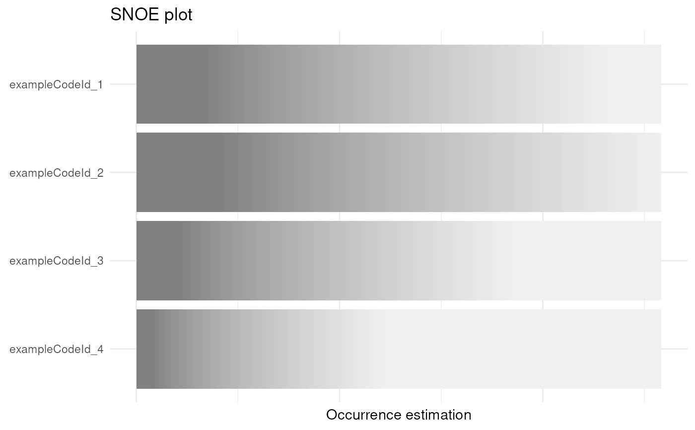
This function produces a Soft Non-numeric Occurrence Estimation plot (a SNOE plot). SNOE plots allow inspection of estimated relative code occurrences without exposing the researcher to proportions, percentages, or frequencies (see the details for an explanation of why this is useful).
Usage
snoe_plot(
  x,
  codes = ".*",
  matchRegexAgainstPaths = FALSE,
  accumulateChildren = TRUE,
  estimateWithin = NULL,
  title = "SNOE plot",
  vertical = FALSE,
  barWidth = 0.9,
  ggplot2Theme = ggplot2::theme_minimal(),
  greyScale = FALSE,
  colors = c("#C0C0C0", "#0072B2"),
  greyScaleColors = c("#C0C0C0", "#808080"),
  silent = rock::opts$get("silent")
)
Arguments
- x
A parsed source(s) object.
- codes
A regular expression to select codes to include, or, alternatively, a character vector with literal code identifiers.
- matchRegexAgainstPaths
Whether to match the
codesregular expression against the full code paths or only against the code identifier.- estimateWithin
The column specifying within what to count.
- title
Title of the plot
- vertical
Whether to plot horizontally (
FALSE, best for reading code- barWidth
The width of the bars; can be decreased or increased, for example in combination with vertical plotting to make the plot look more like a snowy landscape.
- ggplot2Theme
Can be used to specify theme elements for the plot.
- greyScale
Whether to produce the plot in color (
FALSE) or greyscale (TRUE).- colors, greyScaleColors
The (two) colors to use for the color and greyscale versions of the SNOE plot.
- silent
Whether to be chatty or silent
Value
A list containing a ggplot2::ggplot() in the $plot slot.
Details
In qualitative research, sampling is often not random, and data collection is often not systematic. Both of these characteristics are strengths of qualitative research; this flexibility allows optimization of the data collection depending on what is learned, so that rich data can be collected there where it is most informative as to the phenomenon of interest. At the same time, this means that all estimates obtained from qualitative data involve a level of uncertainty that cannot be estimated or modelled (doing so would require either the assumption of random data collection, which does not hold, or the ability to model how the data collection deviates from randomness, which is typically unknown.
This means that when, for example, data have been collected from 40 data providers (e.g., participants), and a given code occurred in 20% of the coded data fragments, it cannot be inferred that the phenomenon or concept represented by this code is more common than another phenomenon or concept, represented by a code that occurred in 20% of the coded data fragments. If the data had been collected identically from a random sample, regular methods could have been used to model the uncertainty, for example by computing confidence intervals, but the width of confidence interval cannot be determined, so it is unclear how much more often a given code has to occur to allow the inference that the corresponding phenomenon or concept occurs more frequently than another phenomenon or concept.
At the same time, such relative statements are often desirable; in fact, next to relationships between phenomena or concept, estimates of relative occurrence are often one of the main epistemological aims of qualitative research. SNOE plots were devised to fill this gap: they visualize the relative occurrence of different codes in a way where the uncertainty is visualized without exposing the researcher to quantified estimates. As a result, code occurrence estimates that are relatively close together are hard to visually distinguish, and only when code occurrence estimates are relatively far apart the code occurrences become visually distinct.
Examples
### Get path to example source
examplePath <-
system.file("extdata", package="rock");
### Get a path to one example file
exampleFile <-
file.path(examplePath, "example-3.rock");
### Load example source
loadedExample <- rock::parse_source(exampleFile);
### Show code occurrence estimates
rock::snoe_plot(
loadedExample
);
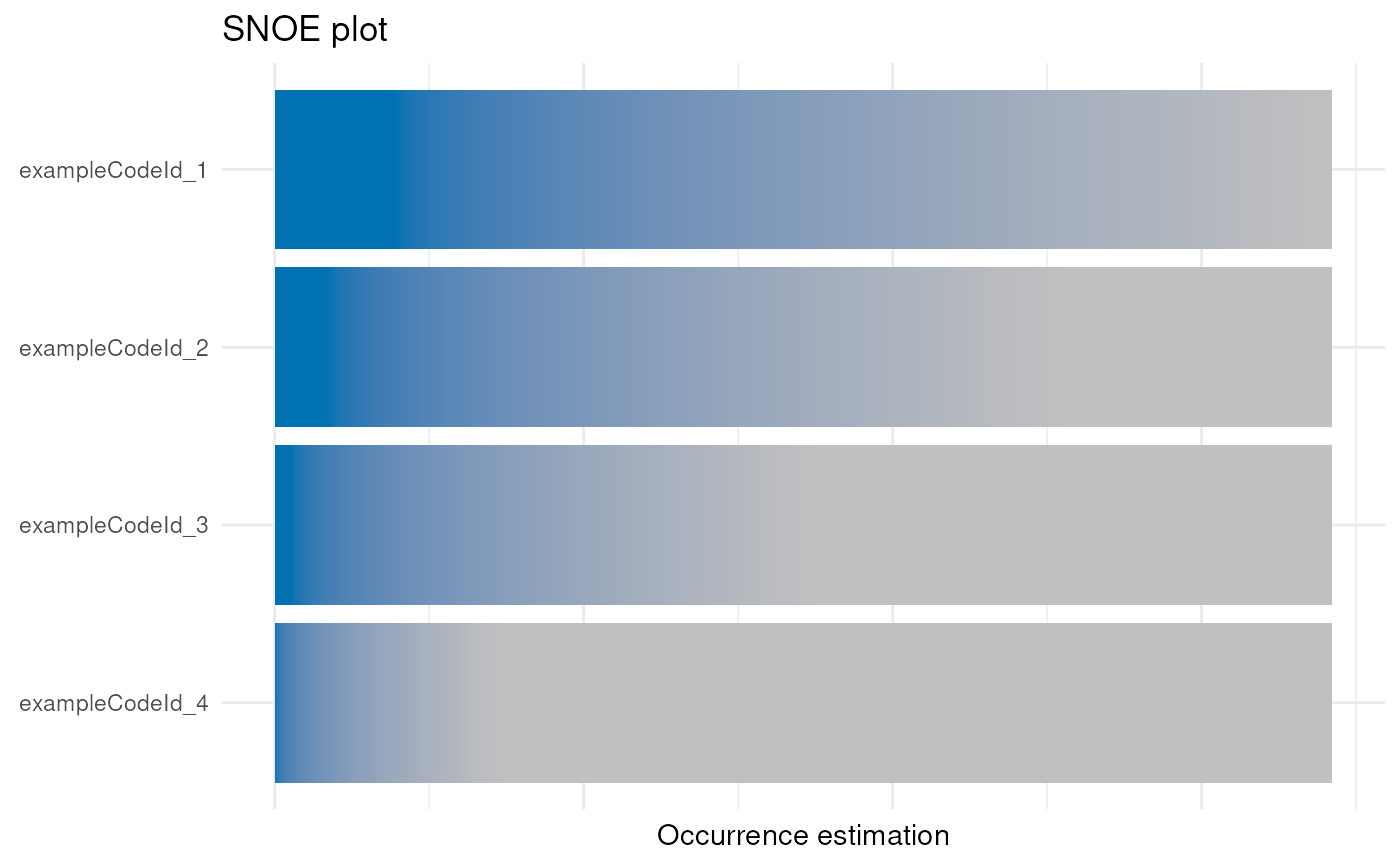 ### Load two example sources
loadedExamples <- rock::parse_sources(
examplePath,
regex = "example-[34].rock"
);
### View the SNOE plot
rock::snoe_plot(
loadedExamples
);
### Load two example sources
loadedExamples <- rock::parse_sources(
examplePath,
regex = "example-[34].rock"
);
### View the SNOE plot
rock::snoe_plot(
loadedExamples
);
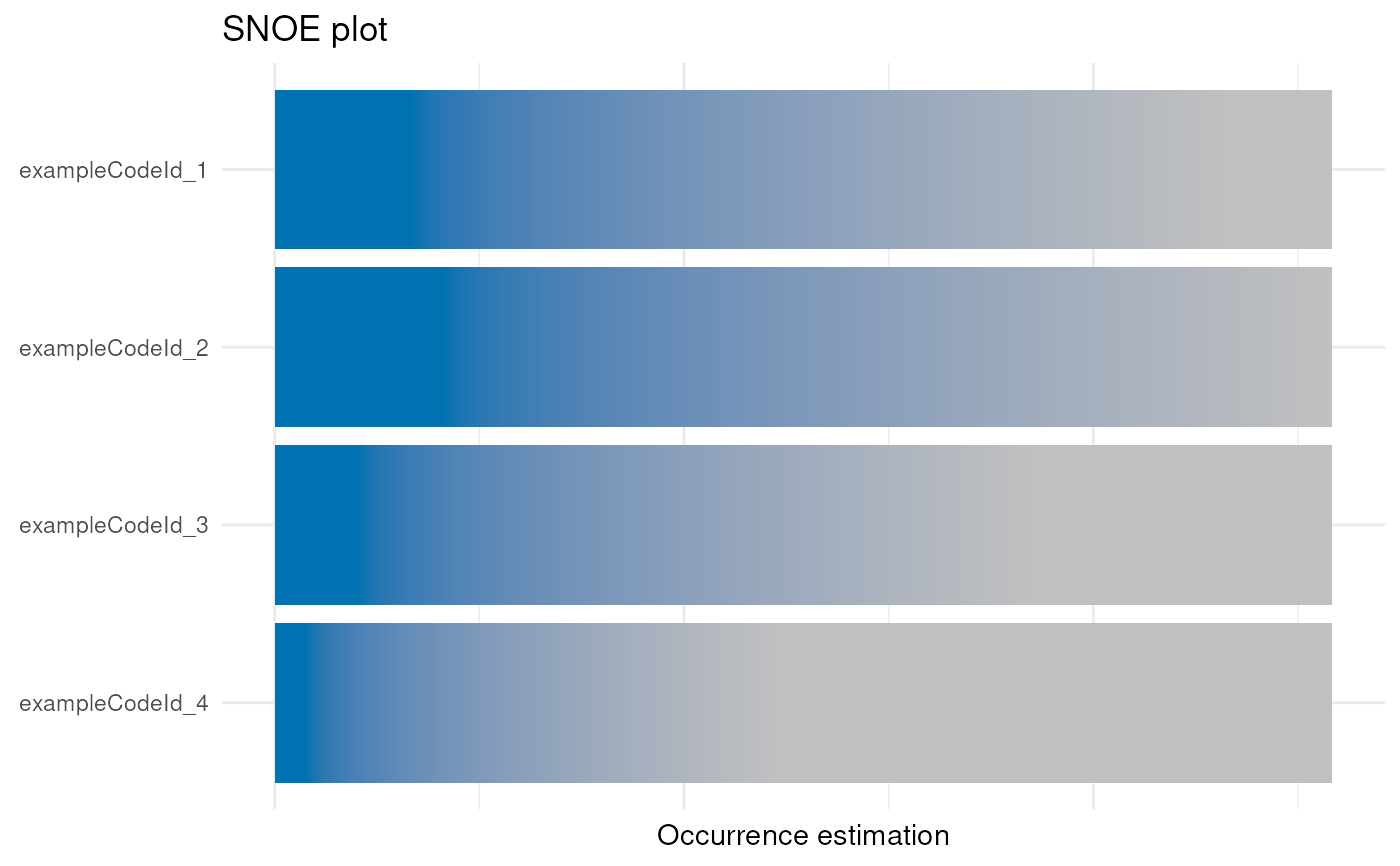 ### For publications, greyscale is recommended:
rock::snoe_plot(
loadedExamples,
greyScale = TRUE
);
### For publications, greyscale is recommended:
rock::snoe_plot(
loadedExamples,
greyScale = TRUE
);
 ### You may want to change the colors to
### increase the contrast:
rock::snoe_plot(
loadedExamples,
greyScale = TRUE,
greyScaleColors =
c("#808080", "#F0F0F0")
);
### You may want to change the colors to
### increase the contrast:
rock::snoe_plot(
loadedExamples,
greyScale = TRUE,
greyScaleColors =
c("#808080", "#F0F0F0")
);
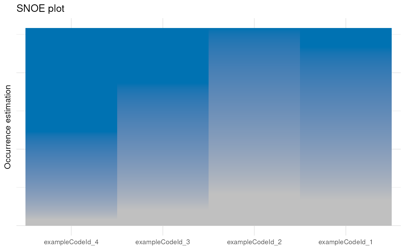
 ### To make the SNOE plot look like snow
### it can be plotted vertically, too. This
### is perhaps not the most *useful* function,
### but it is fun, and fun is important.
rock::snoe_plot(
loadedExamples,
vertical = TRUE,
barWidth = 1
);
### To make the SNOE plot look like snow
### it can be plotted vertically, too. This
### is perhaps not the most *useful* function,
### but it is fun, and fun is important.
rock::snoe_plot(
loadedExamples,
vertical = TRUE,
barWidth = 1
);